KNAPSACK PROBLEM USING BACKTRACKING

KNAPSACK PROBLEM USING BACKTRACKING

This article explains about solving of knapsack problem using backtracking method.

 Concept:

            In solving of knapsack problem using backtracking method we mostly consider the profit but in case of dynamic programming we consider weights.

Concept of backtracking:

            The idea of backtracking is to construct solutions one component at a time and evaluate such partially constructed solutions. This partially constructed solution can be developed further without violating the problem constraints.

            It is convenient to implement this kind of processing by constructing a tree of choices being made called the "State Space Tree". Its root represents an initial state before the search for the solution begins. The nodes of the first level in the tree represent the choices for the first component of a solution and the nodes of a second level represent the choices for the second component and so on.

            A node in the state space tree is promising if it corresponds to the partials constructed solution that may lead to the complete solution otherwise the nodes are called non-promising. Leaves of the tree represent either the non- promising dead end or complete solution found by the algorithm.

 

Concept of Knapsack:

            The knapsack is nothing but a sack where in which we need to place the given items according to the capacity of the knapsack. In case of backtracking we consider the profits but in dynamic programming we consider weights.

 

Algorithm:

            Bound (CP, CW, K)

            {

                        b=CP, c=CW;

                        for i=k+1 to n dp

                        {

                                    c=c + w [i];

                                    if (c<m) then

                                    b= b + p[i];

                                    else

                                    return b+(1-(c-m)/w[i])*p[i]                             ;

                                    return b;

                        }

            }

Consider:

            CP=Current Profit;       CW=Current Weight; K= Index; m=Capacity of Knapsack;

 

Example:

            Profits P1=10, P2=10, P3=12, P4=18.

            Weights W1= 2, W2= 4, W3= 6, W4=9;

            m=15;

            n=4;

           

Tracing:

When,  i=1 C=2; b=10;

When,  i=2 w[2]=4 so, c=c + w[2] c= 2+4= 6  so c= 6 if 6<15  condition gets true so b=10+10=20;

c=6;

b=20

When,  i=3 w[3]=6 so, c=c + w[3] c= 6+6= 12  so c= 12 if 12<15  condition gets true so b=20+12=32;

c=12;

b=32

When,  i=4 w[4]=9 so, c=c + w[4] c= 12+9= 21  so c= 21 if 21<15  condition gets FALSE    so b+(1-(c-m)/w[i])*p[i] is 32+(1-(21-15)/9)*18=38

c=21;

b=38;

Here we got the maximum profit as 38.

To obtain this maximum capacity we need to consider the Item 4 first then Item 2 then Item 1 that is 18+10+10 = 38.

Read more: http://www.articlesbase.com/computers-articles/knapsack-problem-using-backtracking-2099286.html#ixzz1NAexAEAv 
Under Creative Commons License: Attribution

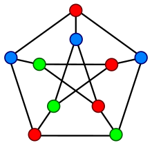
Graph coloring

 In graph theory, graph coloring is a special case of graph labeling; it is an assignment of labels traditionally called "colors" to elements of a graph subject to certain constraints. In its simplest form, it is a way of coloring the vertices of a graph such that no two adjacent vertices share the same color; this is called avertex coloring. Similarly, an edge coloring assigns a color to each edge so that no two adjacent edges share the same color, and a face coloring of a planar graph assigns a color to each face or region so that no two faces that share a boundary have the same color.

Vertex coloring is the starting point of the subject, and other coloring problems can be transformed into a vertex version. For example, an edge coloring of a graph is just a vertex coloring of its line graph, and a face coloring of a planar graph is just a vertex coloring of its planar dual. However, non-vertex coloring problems are often stated and studied as is. That is partly for perspective, and partly because some problems are best studied in non-vertex form, as for instance is edge coloring.

8 queens puzzle

The eight queens puzzle is the problem of placing eight chess queens on an 8×8 chessboard so that no two queens attack each other. Thus, a solution requires that no two queens share the same row, column, or diagonal. The eight queens puzzle is an example of the more general n-queens problem of placing n queens on an n×n chessboard, where solutions exist for all n other than 2 and 3

The problem can be quite computationally expensive as there are 4,426,165,368 (i.e., 64 choose 8) possible arrangements of eight queens on a 8×8 board, but only 92 solutions. It is possible to use shortcuts that reduce computational requirements or rules of thumb that avoids brute force computational techniques. For example, just by applying a simple rule that constrains each queen to a single column (or row), though still considered brute force, it is possible to reduce the number of possibilities to just 16,777,216 (that is, 8⁸) possible combinations. Generating the permutations that are solutions of the eight rooks puzzle^[2] and then checking for diagonal attacks further reduces the possibilities to just 40,320 (that is, 8!). These are computationally manageable for n = 8, but would be intractable for problems of n ≥ 20, as 20! = 2.433 * 10¹⁸. Advancements for this and other toy problems are the development and application of heuristics (rules of thumb) that yield solutions to the nqueens puzzle at a small fraction of the computational requirements.

This heuristic solves N queens for any N ≥ 4. It forms the list of numbers for vertical positions (rows) of queens with horizontal position (column) simply increasing. N is 8 for eight queens puzzle.

1. If the remainder from dividing N by 6 is not 2 or 3 then the list is simply all even numbers followed by all odd numbers ≤ N
2. Otherwise, write separate lists of even and odd numbers (i.e. 2,4,6,8 - 1,3,5,7)
3. If the remainder is 2, swap 1 and 3 in odd list and move 5 to the end (i.e. 3,1,7,5)
4. If the remainder is 3, move 2 to the end of even list and 1,3 to the end of odd list (i.e. 4,6,8,2 - 5,7,9,1,3)
5. Append odd list to the even list and place queens in the rows given by these numbers, from left to right (i.e. a2, b4, c6, d8, e3, f1, g7, h5)

For N = 8 this results in the solution shown above.

	a	b	c	d	e	f	g	h
8									8
7									7
6									6
5									5
4									4
3									3
2									2
1									1
	a	b	c	d	e	f	g	h

One solution.